이산자료의 분석
2018 가을학기 통계학실험 010 강좌
이경원
November 20, 2018
1 (R) list 자료형
- R에는 벡터와 행렬 외에도 list라는 자료형이 있다.
- 벡터와 행렬은 동일한 형식의 원소들을 묶는 자료구조임에 반해, 리스트는 다른 형식의 자료도 묶어주는 자료구조이다. (
data.frame과 거의 비슷하게 작동한다.) - list 자료형의 선언은 다음과 같이 할 수 있다.
## $name
## [1] "Joe"
##
## $salary
## [1] 55000
##
## $union
## [1] TRUE- list 자료형의 구성요소는 다음과 같이 접근할 수 있다.
## [1] 55000## [1] 55000## [1] 55000- 단, 괄호를 하나만 쓰게 될 경우, 부분리스트가 된다.
## $salary
## [1] 55000## $salary
## [1] 55000## $name
## [1] "Joe"
##
## $salary
## [1] 55000- 다음과 같이 벡터나 행렬의 원소를 추가할 수 있다는 것을 알고 있다.
## [1] 1 2 3 4- list도 이와 비슷하게 원소를 추가하거나 합칠 수 있다.
## $a
## [1] "abc"
##
## $b
## [1] 12## $a
## [1] "abc"
##
## $b
## [1] 12
##
## $c
## [1] "sailing"## [[1]]
## [1] "Joe"
##
## [[2]]
## [1] 55000
##
## [[3]]
## [1] TRUE
##
## [[4]]
## [1] 5- 또는 다음과 같이 벡터 인덱스를 이용해 원소를 추가할 수도 있다.
## [[1]]
## [1] 28
##
## [[2]]
## [1] FALSE
##
## [[3]]
## [1] TRUE
##
## [[4]]
## [1] TRUE- 리스트의 원소의 삭제는 다음과 같이 NULL을 입력하는 것으로 시행할 수 있다.
## $a
## [1] "abc"
##
## $c
## [1] "sailing"- 벡터의 길이, 행렬의 차원, 리스트의 크기는 다음과 같이 확인할 수 있다.
## [1] 3## [1] 4 4## [1] 2- 마지막으로, unlist함수는 list를 풀어 벡터 형태로 자료를 출력한다.
##         a         c
## "abc" "sailing"- R에서 많은 함수는 결과값을
list형태로 반환한다. list의 성분을 뽑아내어 함수에서의 결과값을 활용할 수 있다.
df_ex <- data.frame(gr = rep(c(1,2), each = 5), x = 1:10)
test_ex <- t.test(x ~ gr, data = df_ex, var.equal = T)
test_ex$statistic
## t
## -5## [1] 0.0010528262 모비율의 추정과 검정
2.1 이론
- 이항분포 \(B(n,p)\)는 \(n\)이 충분히 크고 \(np,~nq>5\) 일때, 정규분포 \(N(np, npq)\)에 근사한다는 것이 알려져 있다. 이때, \(q=1-p\)이다.
2.2 모비율의 추정
2.2.1 한 모비율에 대한 추정
- 표본 \(X\)가 \(B(n,p)\) 에서의 랜덤표본이라 하자.
- 모비율 \(p\)의 추정량으로는 표본비율 \(\hat{p} = X/n\)을 사용할 수 있다.
- \(X\)가 근사적으로 정규분포 \(N(np, npq)\)를 따르므로 표본비율 \(\hat{p}\)는 근사적으로 정규분포 \(N(p, pq/n)\)을 따른다.
- 따라서 모비율 \(\hat{p}\)에 대한 추론으로 다음의 사실을 사용할 수 있다.
\[Z = \frac{\hat{p}-p}{\sqrt{\hat{p}(1-\hat{p})/n}}\approx \frac{\hat{p}-p}{\sqrt{p(1-p)/n}} \mathrel{\dot{\sim}}N(0,1)\]
2.2.2 두 모비율의 차에 대한 추정
- 표본 \(X_1\), \(X_2\)가 각각 \(B(n_1, p_1),~B(n_2, p_2)\) 에서의 랜덤표본이라 하자.
- 두 모비율의 차 \(p_1 - p_2\)의 추정량으로는 두 표본비율의 차 \(\hat{p}_1 - \hat{p}_2 = \dfrac{X_1}{n_1} - \dfrac{X_2}{n_2}\)를 사용할 수 있다.
- 이때, 정규분포의 성질에 의해 다음이 성립한다.
\[Z = \frac{(\hat{p}_1 - \hat{p}_2)- (p_1 - p_2)}{\sqrt{\hat{p}_1(1-\hat{p}_1)/n_1 + \hat{p}_2(1-\hat{p}_2)/n_2}}\approx \frac{(\hat{p}_1 - \hat{p}_2)- (p_1 - p_2)}{\sqrt{p_1(1-p_1)/n_1 + p_2(1-p_2)/n_2}} \mathrel{\dot{\sim}}N(0,1)\]
2.3 모비율의 검정
2.3.1 한 모비율에 대한 검정
- 표본 \(X\)가 \(B(n,p)\) 에서의 랜덤표본이라 하자.
모비율에 대한 귀무가설 \(H_0:~ p = p_0\)에 대한 표본비율을 이용한 검정은 다음과 같이 실시한다.
- 검정통계량 : \(Z=\dfrac{\hat{p}-p}{\sqrt{\hat{p}(1-\hat{p})/n}}\)
대립가설에 따른 기각역과 검정통계량 \(z_0\)에 대한 유의확률 계산 :
| 가설 | 기각역 | 유의확률 |
|---|---|---|
| \(H_1\): \(p\) > \(p_0\) | \(Z \geq z_{\alpha}\) | \(\mathbb{P}(Z \geq z_0)\) |
| \(H_1\): \(p\) < \(p_0\) | \(Z \leq z_{\alpha}\) | \(\mathbb{P}(Z \leq z_0)\) |
| \(H_1\): \(p \neq p_0\) | \(|Z| \geq z_{\alpha/2}\) | \(\mathbb{P}(|Z| \geq |z_0|)=2 \mathbb{P}(Z \geq |z_0|)\) |
2.3.2 두 모비율의 차에 대한 검정
- 표본 \(X_1\), \(X_2\)가 각각 \(B(n_1, p_1),~B(n_2, p_2)\) 에서의 랜덤표본이라 하자.
두 모비율의 차에 대한 귀무가설 \(H_0:~ p_1 - p_2 = p_0\)에 대한 표본비율을 이용한 검정은 다음과 같이 실시한다.
- 검정통계량 : \(Z=\frac{(\hat{p}_1 - \hat{p}_2)- p_0}{\sqrt{\hat{p}_1(1-\hat{p}_1)/n_1 + \hat{p}_2(1-\hat{p}_2)/n_2}}\)
대립가설에 따른 기각역과 검정통계량 \(z_0\)에 대한 유의확률 계산 :
| 가설 | 기각역 | 유의확률 |
|---|---|---|
| \(H_1\): \(p_1-p_2\) > \(p_0\) | \(Z \geq z_{\alpha}\) | \(\mathbb{P}(Z \geq z_0)\) |
| \(H_1\): \(p_1-p_2\) < \(p_0\) | \(Z \leq z_{\alpha}\) | \(\mathbb{P}(Z \leq z_0)\) |
| \(H_1\): \(p_1-p_2 \neq p_0\) | \(|Z| \geq z_{\alpha/2}\) | \(\mathbb{P}(|Z| \geq |z_0|)=2 \mathbb{P}(Z \geq |z_0|)\) |
\(p_0=0\)일 때는 다음과 같이 합동표본비율 \(\hat{p} = \frac{X_1 +X_2}{n_1+n_2}\)을 이용해 검정을 실시할 수도 있다.
- 검정통계량 : \(Z=\frac{(\hat{p}_1 - \hat{p}_2)}{\sqrt{\hat{p}(1-\hat{p})(1/n_1 + 1/n_2)}}\)
대립가설에 따른 기각역과 검정통계량 \(z_0\)에 대한 유의확률 계산 :
| 가설 | 기각역 | 유의확률 |
|---|---|---|
| \(H_1\): \(p_1-p_2\) > \(p_0\) | \(Z \geq z_{\alpha}\) | \(\mathbb{P}(Z \geq z_0)\) |
| \(H_1\): \(p_1-p_2\) < \(p_0\) | \(Z \leq z_{\alpha}\) | \(\mathbb{P}(Z \leq z_0)\) |
| \(H_1\): \(p_1-p_2 \neq p_0\) | \(|Z| \geq z_{\alpha/2}\) | \(\mathbb{P}(|Z| \geq |z_0|)=2 \mathbb{P}(Z \geq |z_0|)\) |
3 범주형 자료의 분석
- 범주형 자료란 반응변수가 범주형(categorical), 또는 이산형(discrete)인 자료를 뜻한다.
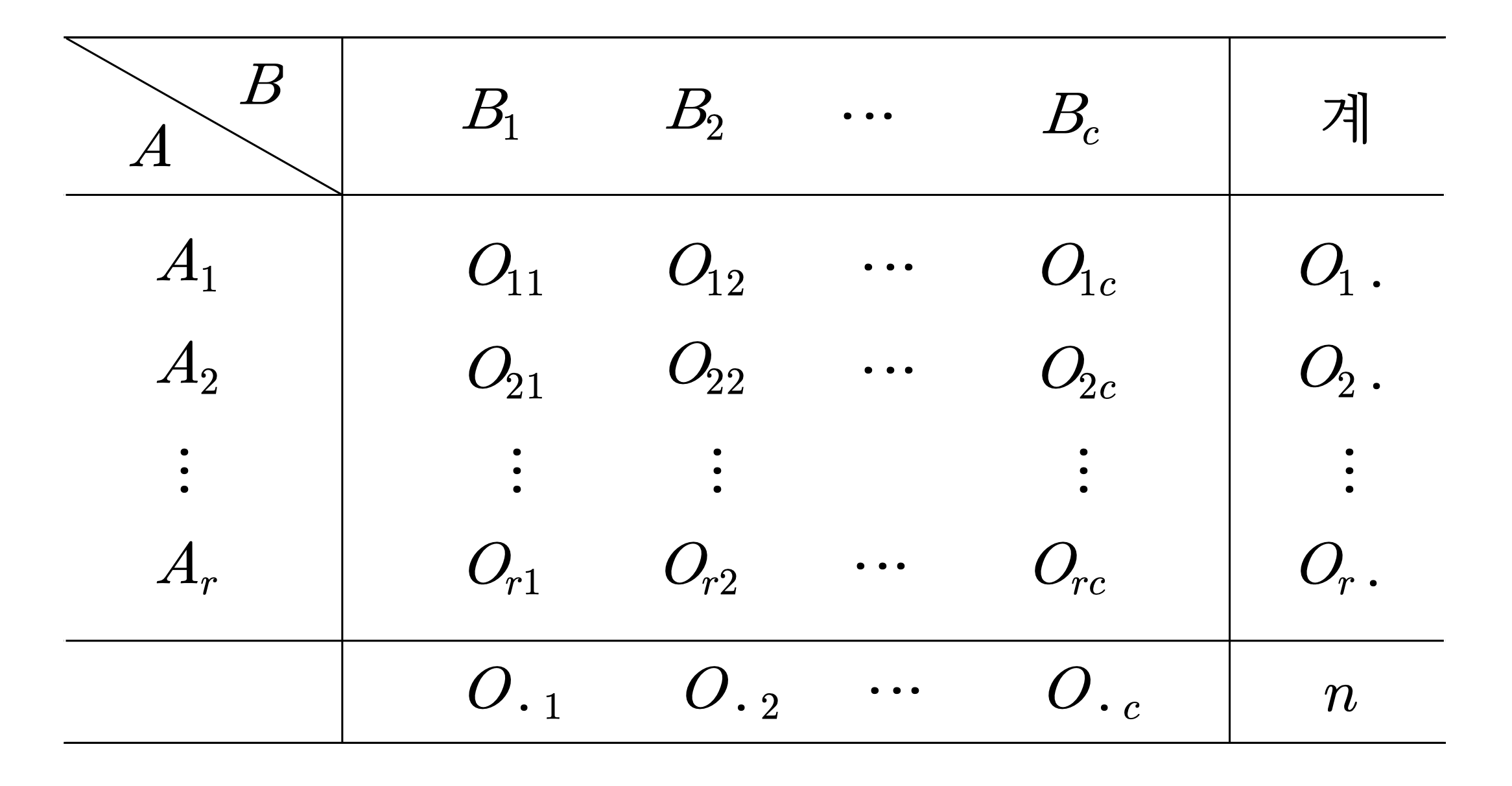
- 범주형 자료는 다음과 같이 분할표(contingency table)을 이용해 나타낸다.
3.1 동질성 검정 (Test of Homogeneity)
3.1.1 동질성 검정
- 동질성 검정이란 “각 모집단이 동질한지 아닌지”를 검정하는 것이다.
- 각 \(i=1,2,\cdots,r\)에 대해 \(n_i = O_{i \cdot}\)라 했을 때, 다항분포를 이용해 \((O_{i1}, \cdots, O_{ic}) \sim Multi(n_i, p_i = (p_{i1}, \cdots, p_{ic}))\) 와 같이 나타낼 수 있다.
- 동질성 검정의 가설은 다음과 같이 나타낼 수 있다.
\[H_0:~p_1 = p_2 = \cdots =p_r, \quad H_1:~\text{not }H_0\]
- 동질성 검정은 검정통계량 \[\chi^2 = \sum_{i=1}^r \sum_{j=1}^c \frac{(O_{ij} - \hat{E}_{ij})^2}{\hat{E}_{ij}}, ~\hat{E_{ij}} = \frac{O_{i\cdot} ~ O_{\cdot j}}{n}\] 을 이용해 실시한다.
- 다음이 성립함이 알려져 있다. \[\chi^2 \mathrel{\dot{\sim}}\chi^2((r-1)(c-1)), \quad \text{under }H_0 \]
- 기각역은 \(\chi^2 \geq \chi^2_\alpha((r-1)(c-1))\)을 사용한다.
- 유의확률은 \(\prob{Z \geq \chi^2 | Z \sim \chi^2((r-1)(c-1))}\)을 사용한다.
- R에서 동질성 검정은
chisq.test()함수를 통해 실시할 수 있다.
3.1.2 예제
- 성별에 따라 국어, 수학, 영어 세 과목의 선호도가 다른가를 조사하고자 한다.
- 남학생 250명과 여학생 250명에 대한 설문조사를 통해 가장 좋아하는 한 과목을 택하게 하여 분류한 결과가 다음과 같다고 하자.
- 남학생과 여학생에 따른 과목의 선호도가 다르다고 할 수 있는지 유의수준 5%에서 검정해보자.
##
##  Pearson's Chi-squared test
##
## data:  x
## X-squared = 36.048, df = 2, p-value = 1.487e-08- 유의수준이 매우 작기 때문에 귀무가설을 기각할 수 있다.
즉, 남학생과 여학생에 따른 과목의 선호도가 다르다고 할 만한 충분한 근거가 있다 말할 수 있다.
다음과 같이 동질성 검정을 실시하는
my_chisq_test()함수를 직접 만들 수 있다.
my_chisq_test <- function(data){
  N = sum(data)
  r = nrow(data)
  c = ncol(data)
  expt = matrix(0, r, c)
  for(i in 1:r){
    for(j in 1:c){
      expt[i, j] <- sum(data[i, ])*sum(data[, j]) / N
    }
  }
  test_stat <- sum((data-expt)^2/expt)
  df = (r-1)*(c-1)
  p.value <- pchisq(test_stat,df,lower.tail=F)
  return(list(statistic = test_stat, df = df,
              p.value = p.value))
}
my_chisq_test(x)
## $statistic
## [1] 36.04756
##
## $df
## [1] 2
##
## $p.value
## [1] 1.48721e-083.2 독립성 검정 (Test of Independence)
3.2.1 독립성 검정
- 독립성 검정이란 “모집단의 각 인자가 독립인지 아닌지”를 검정하는 것이다.
- 다항분포를 이용해 \((O_{11}, \cdots, O_{1c}, \cdots, O_{21}, \cdots, O_{rc}) \sim Multi(n, p = (p_{i1}, \cdots, p_{ic}, \cdots, p_{21}, \cdots p_{rc}))\) 와 같이 나타낼 수 있다.
- 독립성 검정의 가설은 다음과 같이 나타낼 수 있다.
\[H_0:~ p_{ij} = p_{i\cdot}~ p_{j\cdot}~ (i=1,2,\cdots,r, ~j = 1,2,\cdots, c), \quad H_1:~\text{not }H_0\]
- 독립성 검정은 검정통계량 \[\chi^2 = \sum_{i=1}^r \sum_{j=1}^c \frac{(O_{ij} - \hat{E}_{ij})^2}{\hat{E}_{ij}}, ~\hat{E_{ij}} = \frac{O_{i\cdot} ~ O_{\cdot j}}{n}\] 을 이용해 실시한다.
- 다음이 성립함이 알려져 있다. \[\chi^2 \mathrel{\dot{\sim}}\chi^2((r-1)(c-1)), \quad \text{under }H_0 \]
- 기각역은 \(\chi^2 \geq \chi^2_\alpha((r-1)(c-1))\)을 사용한다.
- 유의확률은 \(\prob{Z \geq \chi^2 | Z \sim \chi^2((r-1)(c-1))}\)을 사용한다.
- R에서 독립성 검정은
chisq.test()함수를 통해 실시할 수 있다.
3.2.2 예제
- 이번에는 성별과 과목의 선호도가 독립인지 아닌지를 조사하고자 한다.
- 남학생 250명과 여학생 250명에 대한 설문조사를 통해 가장 좋아하는 한 과목을 택하게 하여 분류한 결과가 다음과 같았다.
- 유의수준 5%에서 검정해보자.
##
##  Pearson's Chi-squared test
##
## data:  x
## X-squared = 36.048, df = 2, p-value = 1.487e-08- 유의수준이 매우 작기 때문에 귀무가설을 기각할 수 있다.
- 즉, 성별과 과목의 선호도가 독립이 아니라고 할 만한 충분한 근거가 있다 말할 수 있다.
3.2.3 주의
- 언뜻 보기에 동질성 검정과 독립성 검정은 서로 같은 검정을 하는 것처럼 보인다.
성별에 따른 과목의 선호도는 차이가 없다 vs 성별과 과목의 선호도는 독립이다
- 그러나, 위의 두 문장에는 큰 차이가 있다.
- 앞의 문장에서는 각 표본의 모집단이 특정 성별의 학생들이고, 뒤의 문장에서는 각 표본의 모집단이 동일하다는 것이 가정되어있다.
- 실제 위의 검정들을 유도하는 것은 서로 다른 가정에서, 다른 계산을 통해 이루어진다.
4 실습
4.1 자료
- 조장은 조원들에게 다음의 정보들을 수집한다.
- 단과대 (“경영대”, “공대”, “기타”)
- 혈액형 (“A”, “B”, “AB”, “O”)
- 탕수육 부먹/찍먹 여부 (“b”: 부먹, “z”: 찍먹)
- R에 다음과 같이 자료를 정리하여 조교의 이메일로 보낸다.
4.2 분석
- 자료는 eTL의 공지사항을 확인하거나 다음의 링크를 클릭해 다운로드 받아 사용하자.
- 다음과 같이 자료를 불러오자.
4.2.1 경영대 학생 비율 추정
- 이 수업에서의 경영대 학생 비율을 이용해 전체 통계학실험 강좌의 경영대 학생 비율을 추정해보자.
- R에서 분할표는
table()함수를 사용해 계산할 수 있다.
##    경영대
## 0.6060606- 약 60% 정도이다.
- 경영대 학생이 전체 통계학실험에서 60% 정도의 비율을 차지고 있다고 말할 수 있다.
무엇이 잘못되었을까?
sampling이 잘 되지 않았다.
4.2.2 동질성 검정
- 경영대와 공대의 A형 혈액형 학생의 비율에 차이가 있는지를 검정해보자.
- 자유도가 낮을 때는 연속성 수정을 실시하기에
correct=F를 사용하여 꺼주자.
##         blood
## college  A AB B O
##   경영대 5  6 4 5
##   공대   4  1 2 3
## 기타 1 0 1 1## Warning in chisq.test(embl_table, correct = F): Chi-squared approximation
## may be incorrect##
## Pearson's Chi-squared test
##
## data: embl_table
## X-squared = 0.71429, df = 1, p-value = 0.398- 학생 비율에 차이가 있다고 말할 수 없다.
동질성 검정? 두 모비율의 차에 대한 검정?
- 두 모비율의 차에 대한 검정을 진행해보자.
prop.test()함수를 사용하면 된다.
## Warning in prop.test(as.matrix(embl_table), alternative = "two.sided",
## correct = F): Chi-squared approximation may be incorrect
##
## 2-sample test for equality of proportions without continuity
## correction
##
## data: as.matrix(embl_table)
## X-squared = 0.71429, df = 1, p-value = 0.398
## alternative hypothesis: two.sided
## 95 percent confidence interval:
## -0.5080624 0.2080624
## sample estimates:
## prop 1 prop 2
## 0.25 0.40- 또는 다음과 같이 수작업으로 실시할 수 있다.
## manually
n_m <- sum(embl_table[1,])
n_e <- sum(embl_table[2,])
p_m <- embl_table[1, 1]/n_m
p_e <- embl_table[2, 1]/n_e
p_tot <- sum(embl_table[,1])/sum(embl_table)
sdme <- sqrt(p_tot * (1-p_tot) * (1/n_e + 1/n_m))
z <- (p_m - p_e) / sdme
z^2
## [1] 0.7142857- 동질성 검정과 같은 결과를 주고 있다는 것을 확인할 수 있다.
- 실제로 통계량을 제곱하면 동질성 검정의 그것과 같다.
4.2.3 독립성 검정
- 탕수육을 먹는 방식과 소속 단과대가 독립인지 아닌지를 검정해보자.
## Warning in chisq.test(table(lec_df[, 2:3]), correct = F): Chi-squared
## approximation may be incorrect
##
## Pearson's Chi-squared test
##
## data: table(lec_df[, 2:3])
## X-squared = 0.059441, df = 3, p-value = 0.9962- 독립이 아니라고 할 만한 충분한 근거가 없다.
과제
조장님들은 안내셔도 됩니다.
Problem 1
- 통계학실험 수강생들 사이에서는 찍먹이 부먹보다 우세한지 아닌지를 유의수준 5% 에서 검정해보려 한다.
- 다음 물음에 답하여라.
- 찍먹 학생들의 비율을
prob_z, 부먹 학생들의 비율을prob_b변수에 저장하여라.
##         z
## 0.6969697## b
## 0.3030303- 가설을 검정하기 위한 검정통계량을
stat_zb변수에 저장하여라.
- 찍먹 학생들의 모비율을 \(p_1\) 라 하자.
- 검정하고자 하는 가설은 다음과 같다. \[H_0: p_1 = 1/2, \quad H_1: p_1 >1/2\]
- 검정통계량을 다음과 같이 계산할 수 있다.
##        z
## 2.462104- (참고) 검정통계량을 다음과 같이 계산할 수도 있다.
##       z
## 2.26301- 가설을 검정하기 위한 유의확률을
p_zb변수에 저장하여라.
- 귀무가설 하에서
stat_zb는 정규분포를 따르므로 유의확률은 다음과 같이 계산할 수 있다.
##           z
## 0.006906229- 검정 결과를 주석의 형태로 작성해보아라.
- 유의확률이 0.05보다 작으므로 귀무가설을 기각할 수 있다.
- 즉, 찍먹이 부먹보다 우세하다고 할 만한 충분한 근거가 있다.
(참고) 이 문제를 “두 모비율의 차에 대한 검정”으로 풀어서는 안된다. 전체 표본의 수를 \(n\), 찍먹 학생들의 수를 \(n_1\), 부먹 학생들의 수를 \(n_2\)라 하자. 이때, \[Cov(n_1,n_2) = Cov(n_1,n-n_1) = -Var(n_1) \neq 0\]이므로 표본비율 \(\hat{p}_1\), \(\hat{p}_2\)는 절대 독립이 될 수 없다. 따라서, 표본 \(n_1\), \(n_2\)가 서로 독립인 두 이항분포에서의 표본이라 말할 수 없고, 두 모비율의 차에 대한 검정을 적용할 수 없다.
Problem 2
- 단과대별로 혈액형 구성이 다른지를 유의수준 5%에서 검정해보려 한다.
- 가설을 검정하기 위한 검정통계량을
stat_abc변수에 저장하여라.
- 검정하고자 하는 가설은 동질성 가설로, 검정통계량으로는 카이제곱통계량을 사용할 수 있다.
chisq.test()의 검정통계량을 추출할 수 있다.
## Warning in chisq.test(table_abc): Chi-squared approximation may be
## incorrect## X-squared
## 2.79627- 가설을 검정하기 위한 유의확률을
p_abc변수에 저장하여라.
chisq.test()의 유의확률을 추출할 수 있다.
## [1] 0.8339483- 검정 결과를 주석의 형태로 작성해보아라.
- 유의확률이 크므로 귀무가설을 기각할 수 없다.
- 즉, 단과대별로 혈액형의 구성이 다르다고 할 만한 충분한 근거가 없다.